Calculating Impervious Surface Area

Introduction

For this week we were supposed to learn how to Classify aerial images to determine various surface types. This was done through an Online tutorial at ESRI's webpage, found here.

Since many impervious surfaces are a danger, many governments charge landowners that have high amounts of impervious surfaces on their properties. To calculate fees it is important to segment and classify aerial imagery by land and calculate the area of impervious surfaces per land parcel. To decide which parts of the ground are pervious and which one are impervious, one has to classify the imagery into land types. Typically, impervious surfaces are generally human-made such as buildings, roads or parking lots. To start with, change the band combinations to distinguish features clearly. After that one shall group pixels into different segments, which will reduce the number of spectral signatures to classify.

The map includes a feature class of land parcels and a 4-band aerial photograph of an area near Louisville, Kentucky.

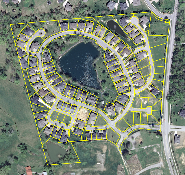Figure 1: A neighborhood near Louisville, Kentucky.

Right now, the imagery uses the natural color band combination to display the imagery the way the human eye would see it. Next step is to change this band combination to better distinguish urban features such as concrete from natural features such as vegetation.

Figure 2: Raster Functions

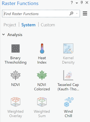Figure 3: Other Raster Functions options, not used here.

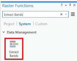Figure 4: Extract bands

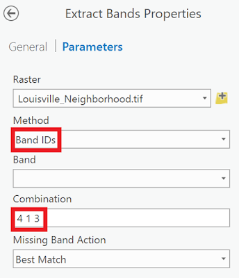Figure 5: Changing band combination

The result displayed below.

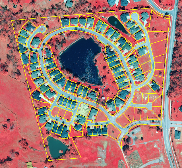Figure 6: The results and the parcels included

The new layer displays only the extracted bands. In order to make some features easier to see, I will turn the yellow parcel layer off.

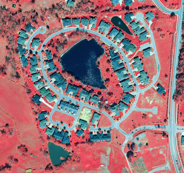Figure 7: Without the parcel layer

Vegetation appears as red, roads as gray, and roofs as shades of gray/blue-ish. It will be easier to classify the surfaces later when emphasizing the difference between natural and human-made surfaces.

Make sure that the Extract_Bands_Louisville_Neighborhoods layer is selected, then select the Classification Wizard.

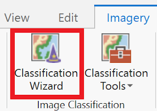Figure 8: Start the Classification Wizard

This time, I will use supervised classification method. This method is based on user-defined training samples. Also, I will use an object based classification which uses a process called segmentation to group neighboring pixels based on the similarity of their spectral characteristics.

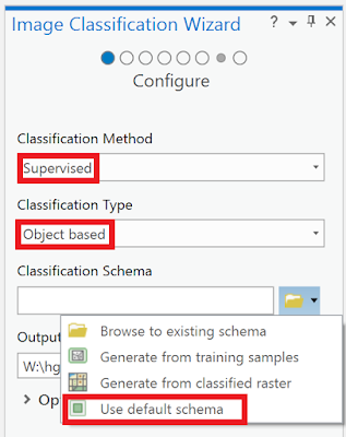Figure 9: First step in the Classification Wizard

Next step is to segment the image. Instead of classifying thousands of pixels with unique spectral signatures, it saves time and storage to classify a much smaller number of segments. Mainly, there are three parameters to take care of: the spectral detail, the spatial detail and the minimum number of segment size in pixels. As instructed I use these number below.

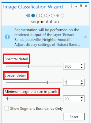Figure 10: Second step in the Classification Wizard

Especially on the left side of the image, vegetation seems to have been grouped into many segments that blur together.

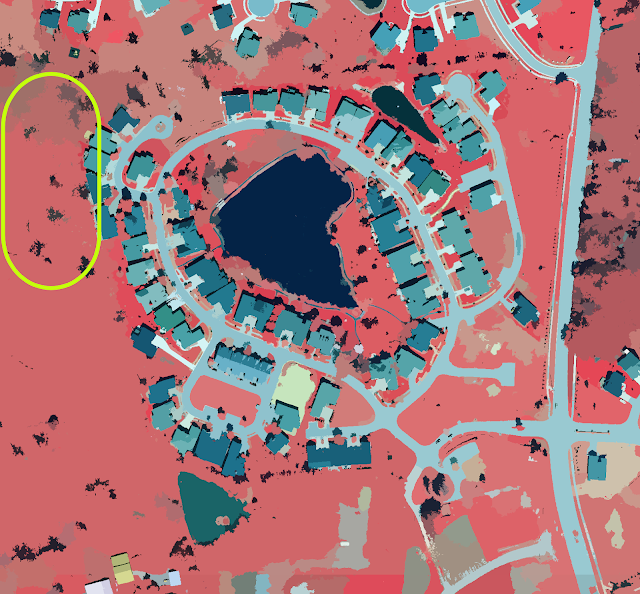Figure 11: Segmented result

This image is being generated on the fly, which means the processing will change based on the map extent, if it is zoomed in or out. At full extent, the image is generalized to save time. The image below is zoomed in to reduce the generalization. By doing so, one can better see what the segmentation looks like.

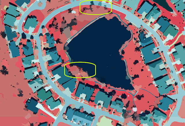Figure 12: Some differences

I have now extracted spectral bands to emphasize the distinction between pervious and impervious features. Then I grouped the pixels with similar spectral characteristics into segments, simplifying the image so that features can be more accurately classified. After these steps, I will classify the imagery by different levels of perviousness or imperviousness. When classified the segmented image into only pervious and impervious surfaces, the classification would be too generalized and likely have many errors. By classifying the image based on more specific land-use types, the classification becomes more accurate.

I put in the numbers once more. On the Training Samples Manager page of the Classification wizard, I right-clicked each of the default classes and remove them. And added some new classes with new values.

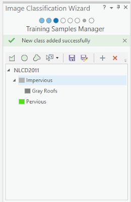Figure 13: Third step in the Classification Wizard

On some roofs I drew polygons and made sure the polygons covered only the pixels that comprise the roofs.

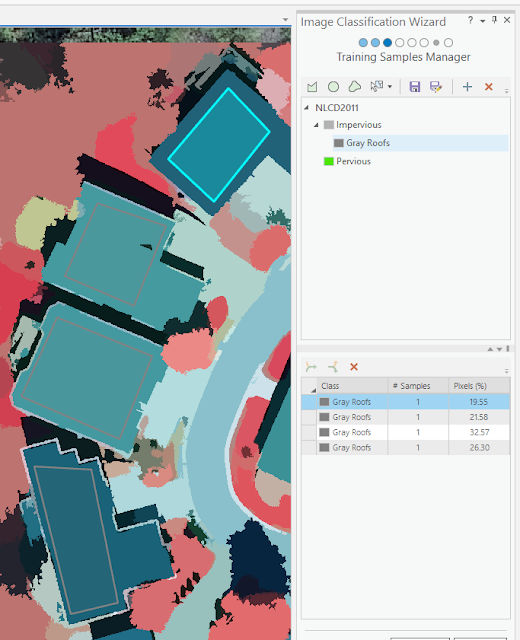Figure 14: Drawing polygons

I have only drawn training samples on roofs, each training sample currently exists as its own class. I want all gray roofs to be classified as the same value, so I will merge the training samples into one class. I selected every training sample and clicked the Collapse button below.

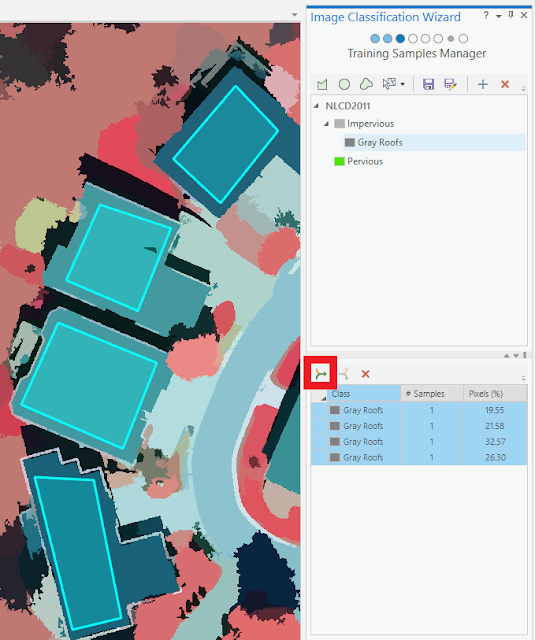Figure 15: Collapse button demonstrated

After creating the different feature classes I did went looking on the map for every one of them
.

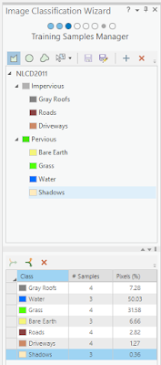Figure 16: Finishing third step

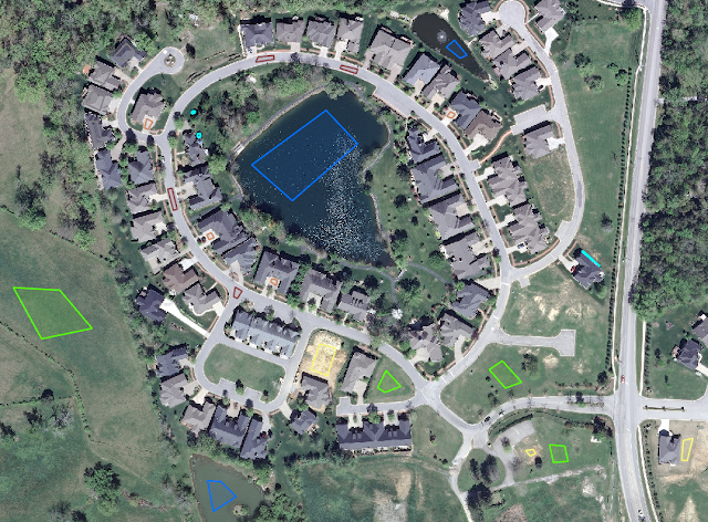Figure 17: The normal view with the polygons I created

When satisfied after finishing my training samples, it is important to save the editing. Next phase is to choose classification method. I will use the so-called Support Vector Machine.

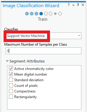Figure 18: Fourth step in the Classification Wizard

On the map is a preview of the classification I just made. The classification preview is pretty accurate, even the muddy pond central bottom was classified correctly. However, it is pretty rare that every feature will be classified correctly.

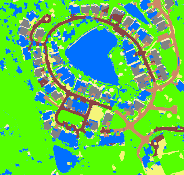Figure 19: The classification preview

Next thing to do is to merge subclasses into their parent classes. I will merge subclasses into Pervious and Impervious parent classes to create a raster with only two classes.

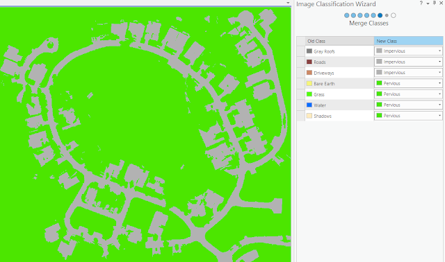Figure 20: Fifth step in the Classification Wizard

The final page of the wizard is the Reclassifier page, which holds tools for reclassifying minor errors in the raster dataset. I uncheck all the layers except the recent one created Preview_Reclass and the base Louisville_Neighborhood.tif layer. The image below shows how some roof tops was not correctly classified. However, the tool is used for when one wants to reclassify a whole area (the polygon). Since I do not want to reclassify this whole area to either pervious nor impervious I just skip this step.

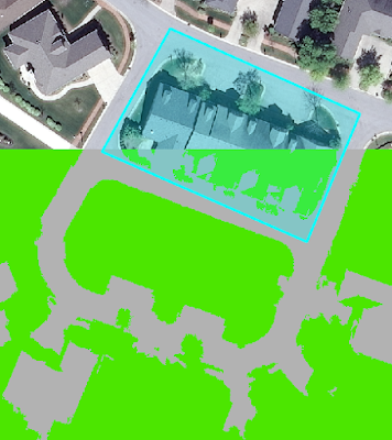Figure 21: Option to reclassify, if wanted

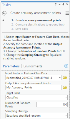Figure 22: Creating assessment points

Conclusions

One hundred accuracy points are added to the map and the tolls added attributes to the points. The points attribute table contains the class value of the classified image for each point location. Next step is to use the accuracy points data to compare the classified image to the ground truth of the original image. After some computations this is the results I ended up with. The parcels with the highest area of impervious surfaces appear to be the ones that are red and correspond to the location of roads. These parcels are very large and almost entirely impervious and larger parcels often have larger impervious surfaces.

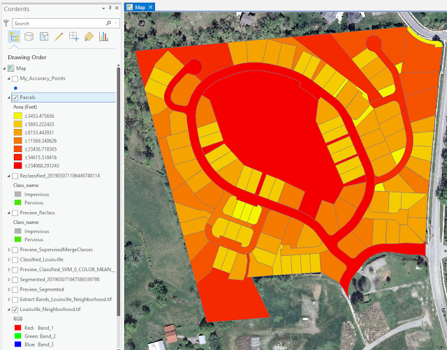Figure 23: After some computations this is the results I ended up with

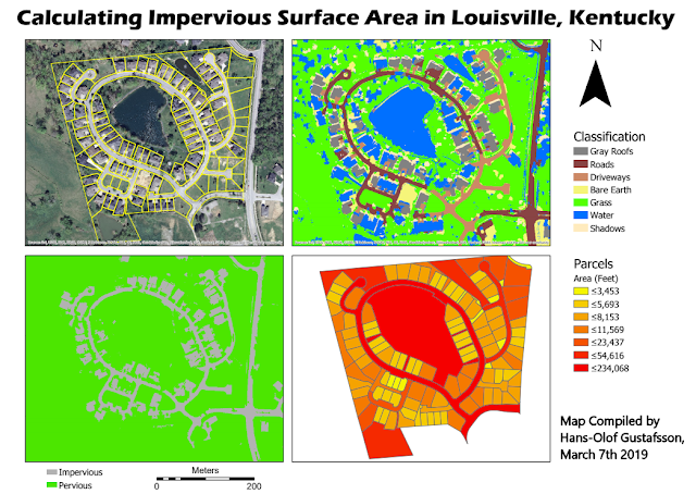Figure 24: The map I created, displaying all the steps of the classification and calculations

Manifold industries and companies can get their business's growing by using UAS data to calcuate perviousness and imperviousness. When planning sites for buildings or different structures this tool would be good to use. Also, this is a good tool for accurately show how land areas changes over time, which may be used by people with other interest. Information collected by UAVs can be used to so many things, this was just another example.